This past February, the sports world witnessed one of the most improbable comebacks in history. The New England Patriots rallied from a 28-3 deficit to beat the Atlanta Falcons and win the NFL Super Bowl. Right now, hockey fans are being treated to one of the most entertaining NHL postseasons ever. The 2017 playoffs have set a record with 18 first round overtime games. On the other hand, the 2017 NBA Playoffs have drawn some criticism as the lack of parity this year has lead to the inevitable third straight Cleveland Cavaliers vs. Golden State Warriors Finals matchup. The Warriors went 12-0 against the Western Conference with an average margin of victory of 16.3 points, per ESPN Stats and Info. The Cavaliers won 12 of 13 games against the Eastern Conference, with all four of their wins over the Boston Celtics coming by at least 13 points, including this record breaking lopsided affair.
These recent events triggered a question primed for a data-based answer, which league (NBA, NHL, NFL, or MLB) is the most competitive?
In this post, I propose an empirical method for comparing competitiveness across leagues. I measured competitiveness by looking at:
- Which league is most likely to produce a comeback game?
- Which league is most likely to produce a close game?
- Which league is most likely to produce a blowout game?
- Which league has the most linear relationship between wins and payroll?
- Which league is the most predictable?
Click here to the jump to final competitiveIndex calculation.
In this analysis, I utilized an expansive sports data API, powered by Stattleship, to get historical game data and game scores by quarter. I also scraped Sports Reference for team payroll data.
The R code used for data wrangling and analysis can be found here for the NBA, NHL, NFL, and MLB.
First, in order to measure the likelihood of comebacks, close games, and blowouts, I used the granular box score data to calculate game score differentials at each quarter/inning/intermission break for all regular season and playoff games since 2015. I then used these score differentials to determine if a game fit one of the categories.
Comebacks
I define comebacks by two cases:
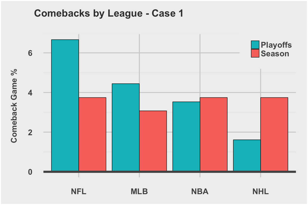
Case 1: Team is down by X points going into the final quarter and ends up wining the game.
Case 2: Team is down by X points going into halftime and ends up winning the game.
To determine an appropriate X point threshold to qualify a ‘comeback’, I looked at the average deficit going into the final quarter for a team who ultimately lost the game.
| League | X Threshold |
|---|---|
| NBA | 9 points |
| NHL | 1 goal |
| NFL | 9 points |
| MLB | 2 runs |
Example Comeback Game:
Box Score
| Game | Team | Q1 | Q2 | Q3 | Q4 | OT | Final |
|---|---|---|---|---|---|---|---|
| Super Bowl 51 | New England Patriots | 0 | 3 | 6 | 19 | 6 | 34 |
| Super Bowl 51 | Atlanta Falcons | 0 | 21 | 7 | 0 | 0 | 28 |
Calculated Game Score Differentials
| Game | Team | DeltaQ1 | DeltaQ2 | DeltaQ3 | DeltaQ4 | DeltaFinal |
|---|---|---|---|---|---|---|
| Super Bowl 51 | New England Patriots | 0 | -18 | -19 | 0 | 6 |
| Super Bowl 51 | Atlanta Falcons | 0 | 18 | 19 | 0 | -6 |
This game would qualify as both case 1 and case 2 comebacks since the Patriots were down by 18 points at halftime and 19 points going into the 4th but still won the game. Now let’s look at the likelihood of a comeback game across the 4 leagues.
Case 1: Down by Xpts going into final quarter and win
Case 2: Down by Xpts going into halftime and win
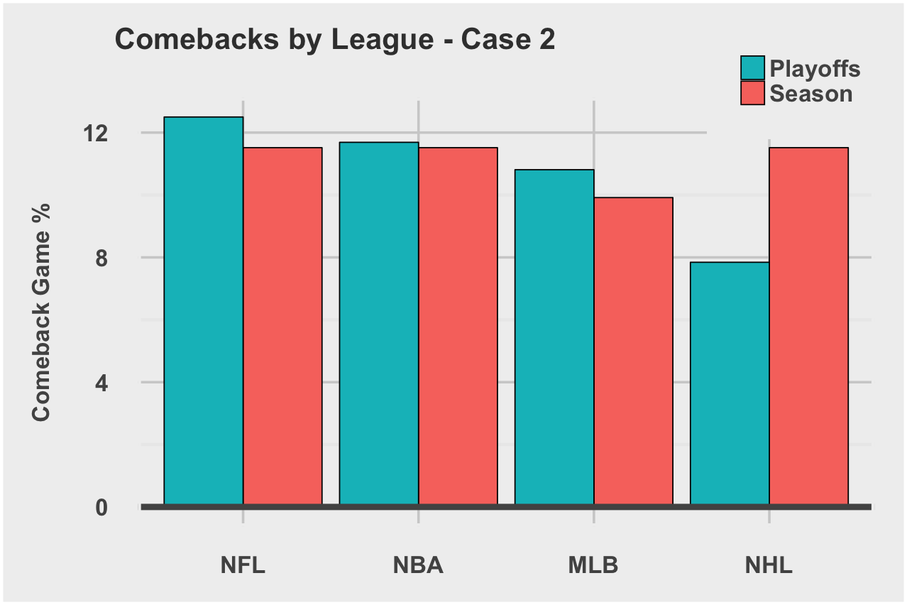
Overall, the likelihood of a comeback game is small across the leagues. There aren’t any clear signals. I average the comeback game rates for regular season, playoffs, and both cases to arrive at a Global Comeback Rate. We’ll use this rate later in the final competitiveIndex calculation.
| League | Global Comeback Rate |
|---|---|
| NFL | 8% |
| NBA | 7.4% |
| MLB | 7.1% |
| NHL | 5.6% |
Close Games
I define close games by three cases:
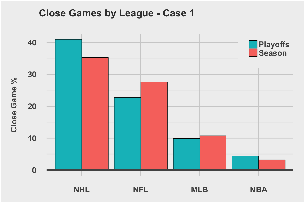
Case 1: The game is within Y points through each quarter and final score is within Y points (or game goes to OT).
Case 2: The game is within Y points going into the final quarter and final score is within Y points (or game goes to OT).
Case 3: The final score is within Y points (or game goes to OT).
For the Y point threshold to qualify a ‘close game’, I chose the maximum scorable points on one possession.
| League | Y Threshold |
|---|---|
| NBA | 4 points |
| NHL | 1 goal |
| NFL | 8 points |
| MLB | 1 run |
Example Close Game:
For our close game example, I chose the epic back-n-forth NBA Finals Game 7 (aka the undercard to Game of Thrones’ Battle of the Bastards which aired right after).
Box Score
| Game | Team | Q1 | Q2 | Q3 | Q4 | Final |
|---|---|---|---|---|---|---|
| 2016 NBA Finals Game 7 | Golden State Warriors | 22 | 27 | 27 | 13 | 89 |
| 2016 NBA Finals Game 7 | Cleveland Cavaliers | 23 | 19 | 33 | 18 | 93 |
Calculated Game Score Differentials
| Game | Team | DeltaQ1 | DeltaQ2 | DeltaQ3 | DeltaQ4 | DeltaFinal |
|---|---|---|---|---|---|---|
| 2016 NBA Finals Game 7 | Golden State Warriors | -1 | 7 | 1 | -4 | -4 |
| 2016 NBA Finals Game 7 | Cleveland Cavaliers | 1 | -7 | -1 | 4 | 4 |
This game would qualify as both case 2 and case 3 close games since the game score differential going into the final quarter and final score were within 4 points. However, because the halftime score differential was 7 points, I am not qualifying this game as a case 1 close game. Now let’s look at the likelihood of a close game across the 4 leagues.
Case 1: Game is within Y points through each quarter and final score (or OT)
Case 2: Game is within Y points going into final quarter and final score (or OT)
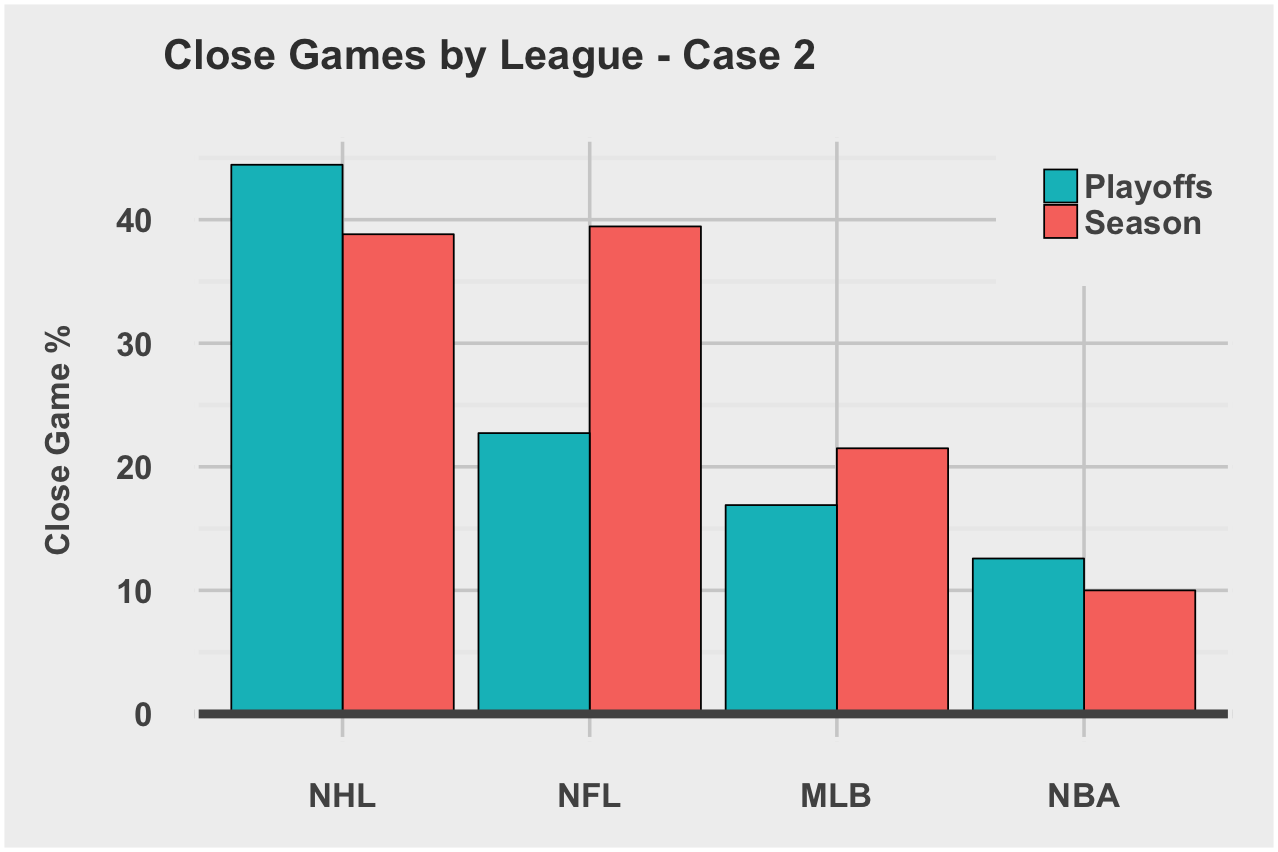
Case 3: Game’s final score is within Y points (or OT)
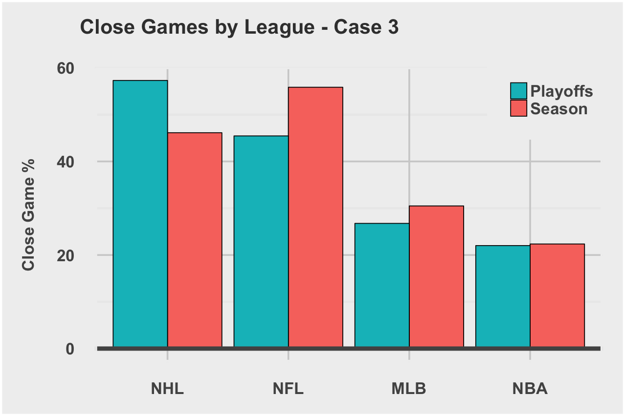
The NHL and NFL stand out as most likely to produce close games. I average the close game rates for regular season, playoffs, and all three cases to arrive at a Global Close Game Rate. We’ll use this rate later in the final competitiveIndex calculation.
| League | Global Close Game Rate |
|---|---|
| NHL | 43.7% |
| NFL | 35.6% |
| MLB | 19.4% |
| NBA | 12.5% |
Blow Outs
I define blowouts by three cases:
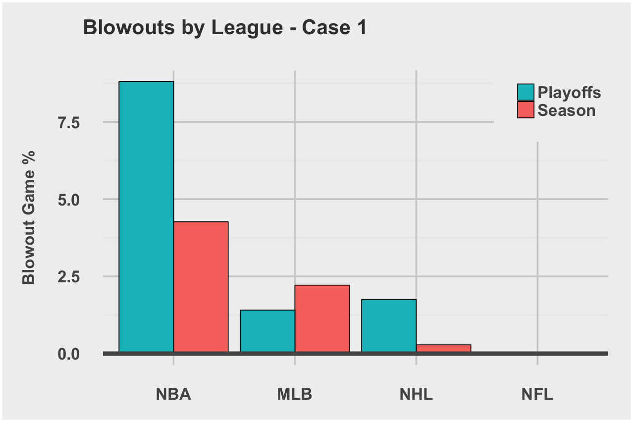
Case 1: The game score deficit is greater than Z points through each quarter and final score deficit is greater than Z points.
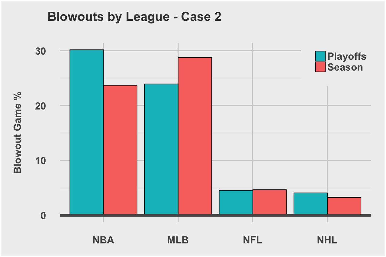
Case 2: The game score deficit is greater than Z points going into the final quarter and final score deficit is greater than Z points.
Case 3: The final score deficit is greater than Z points.
For the Z point threshold to qualify a ‘blowout game’, I chose three times the maximum scorable points on one possession.
| League | Z Threshold |
|---|---|
| NBA | 12 points |
| NHL | 3 goals |
| NFL | 24 points |
| MLB | 3 runs |
Example Blowout Game:
Box Score
| Game | Team | Q1 | Q2 | Q3 | Q4 | Final |
|---|---|---|---|---|---|---|
| 2017 NBA Playoffs | Boston Celtics | 18 | 13 | 26 | 29 | 86 |
| 2017 NBA Playoffs | Cleveland Cavaliers | 32 | 40 | 31 | 27 | 130 |
Calculated Game Score Differentials
| Game | Team | DeltaQ1 | DeltaQ2 | DeltaQ3 | DeltaQ4 | DeltaFinal |
|---|---|---|---|---|---|---|
| 2017 NBA Playoffs | Boston Celtics | -14 | -41 | -46 | -44 | -44 |
| 2017 NBA Playoffs | Cleveland Cavaliers | 14 | 41 | 46 | 44 | 44 |
This game would qualify as case 1, case 2, and case 3 blowouts since the game differentials are all greater than 12 points… by a mile. Now let’s look at the likelihood of a blowout game across the 4 leagues.
Case 1: Game score differential is greater than Z points through each quarter and final score
Case 2: Game score differential is greater than Z pts into the final quarter and final score
Case 3: Game final score differential is greater than Z points
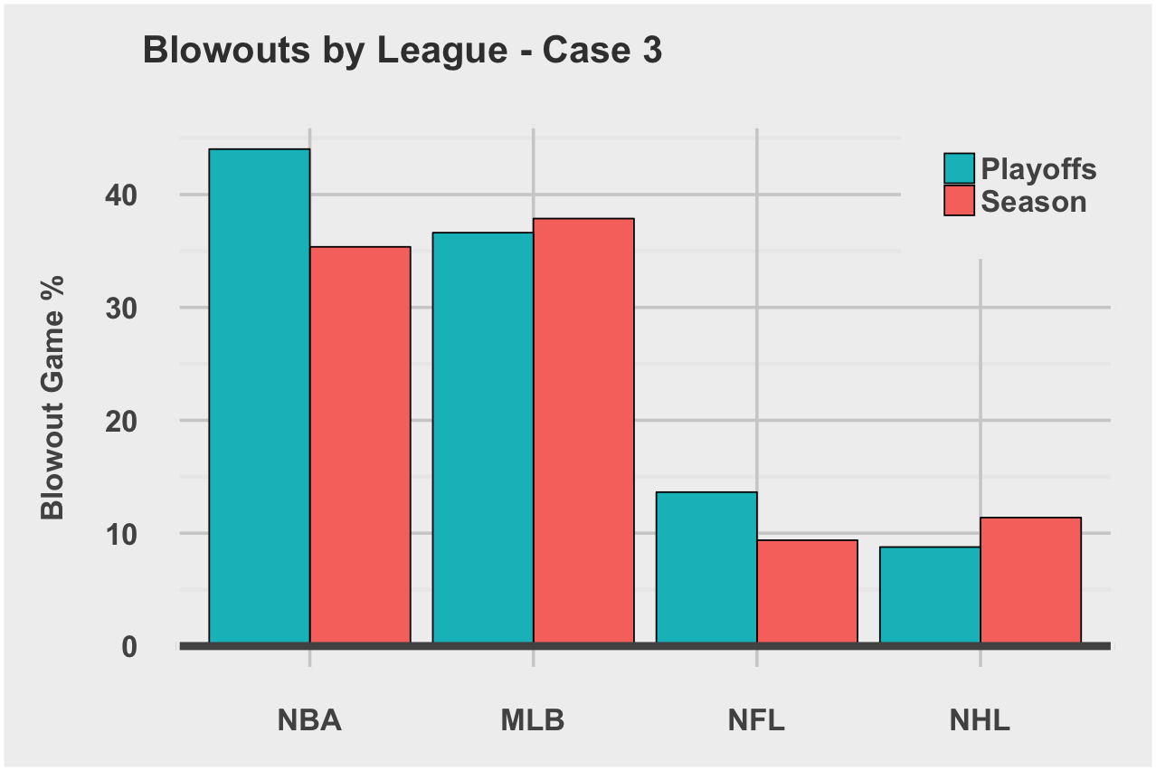
The NBA and MLB stand out as most likely to produce blowout games. I average the blowout rates for regular season, playoffs, and all three cases to arrive at a Global Blowout Game Rate. We’ll use this rate later in the final competitiveIndex calculation.
| League | Global Blowout Rate |
|---|---|
| NBA | 24.2% |
| MLB | 21.8% |
| NFL | 5.4% |
| NHL | 4.9% |
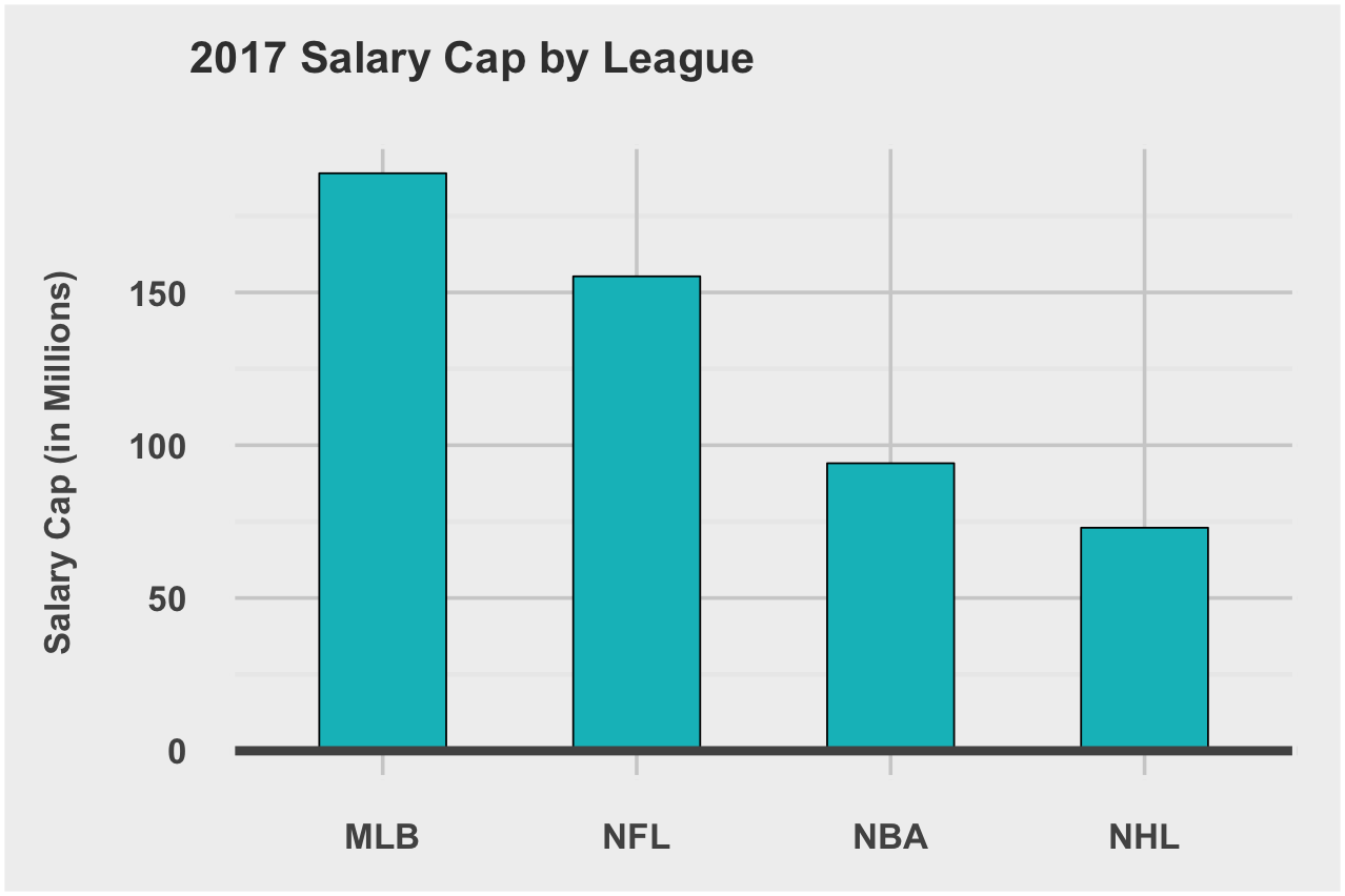
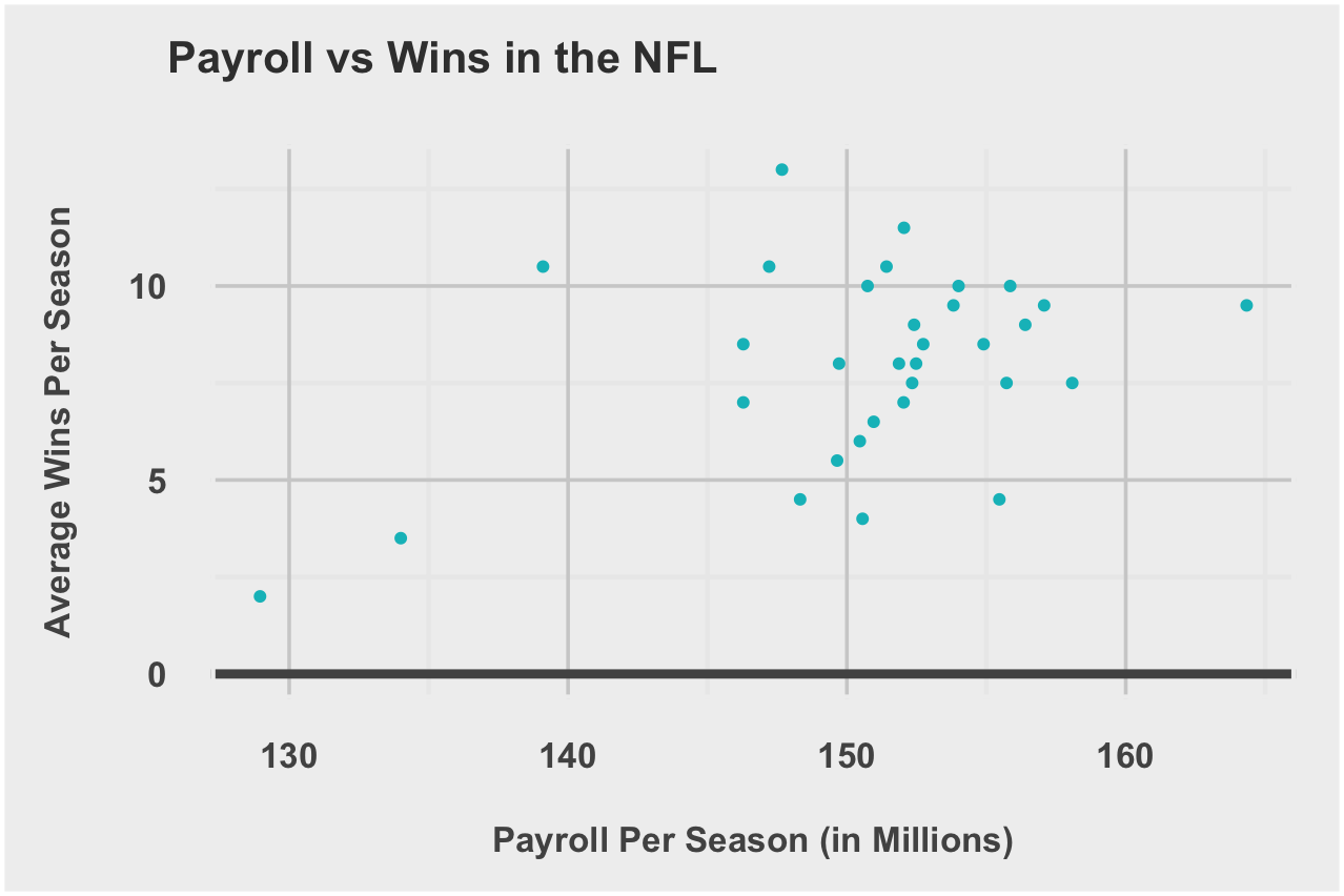
Salary Cap
Salary caps were introduced to the NBA, NHL, and NFL over the last three decades with the goal to reduce the competitive imbalance between bigger spending, large market clubs and the lower revenue, smaller market clubs. The NHL and NFL’s caps are considered “hard”, meaning that they offer relatively few (if any) circumstances under which teams can exceed the salary cap. The NBA features a “soft” cap, meaning that there are several significant exceptions that allow teams to exceed the salary cap to sign players. In place of a salary cap, the MLB implemented a luxury tax, which allow teams to spend as much as they want on salary, but it penalizes them a percentage of the amount by which they exceed a threshold.
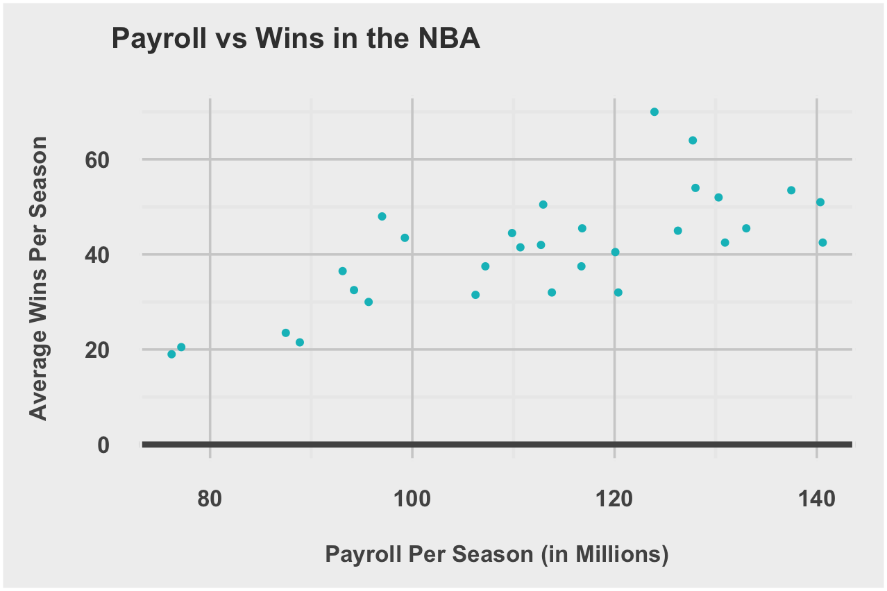
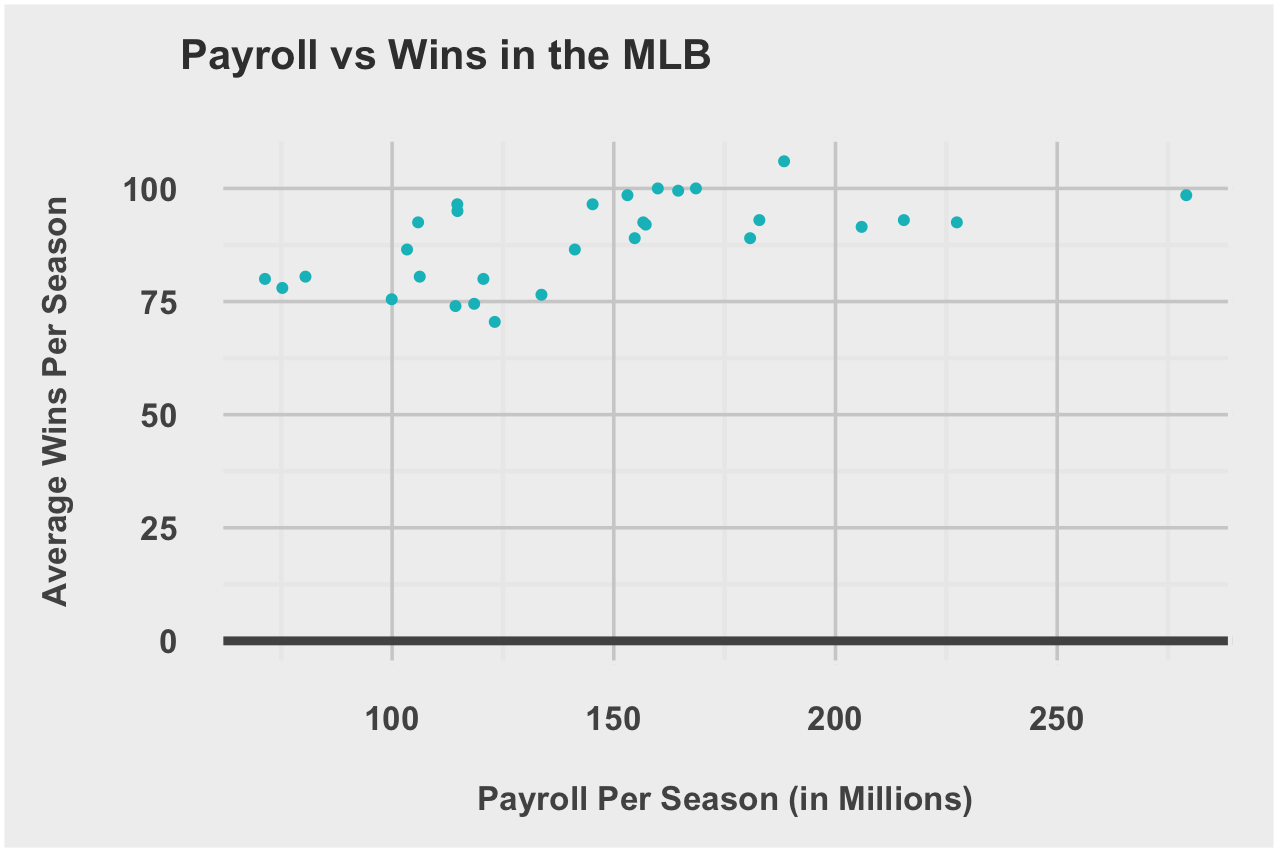
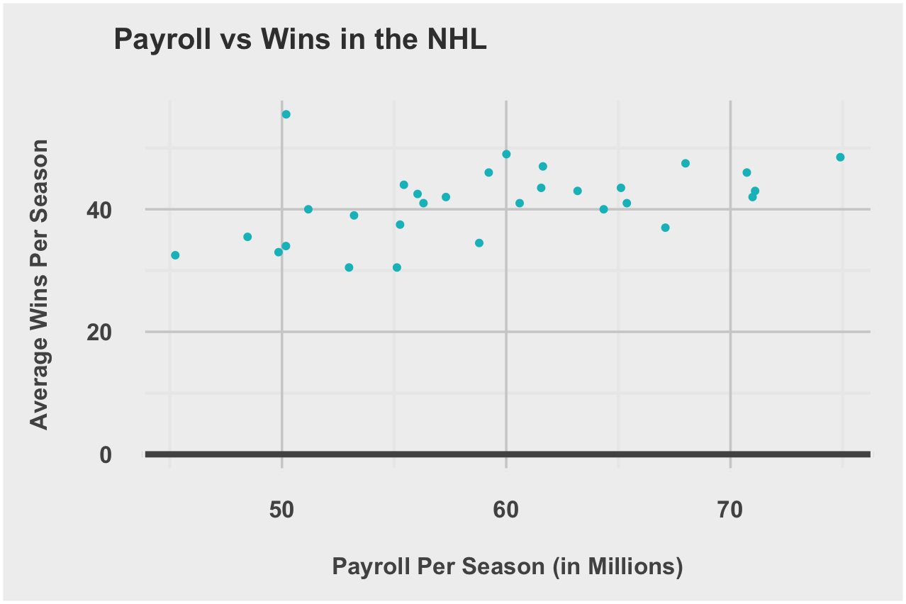
I scraped the latest payroll numbers for every team across the four leagues, to determine the correlation between total wins in a season and a team’s payroll for that season. We will use these correlations in our own competitiveIndex calculation of parity in sports.
Using R’s correlation function, I calculated the relationship between wins and salary.
Score of 1 means perfect linear relationship
Score of 0.7 means strong linear relationship
Score of 0.5 means moderate linear relationship
Score of 0.3 means weak linear relationship
Score of 0 means no relationship
SalaryWinCorrelation = 0.7262808
SalaryWinCorrelation = 0.5943053
SalaryWinCorrelation = 0.4539921
SalaryWinCorrelation = 0.4083673
Hard cap leagues do have a weaker correlation between salary and wins, good sign for parity in the NFL and NHL. We’ll use this correlation later in the final competitiveIndex calculation.
| League | SalaryWinCorrelation |
|---|---|
| NBA | 0.7262808 |
| MLB | 0.5943053 |
| NHL | 0.4539921 |
| NFL | 0.4083673 |
Predictive Modeling
The final variable in our competitiveIndex calculation will be a measure of predictability across the leagues. In this part of the analysis, I look to predict Case 3 blowouts for the NBA and MLB and Case 3 close games for the NFL and NHL. These were the most likely cases for each league and will provide the largest sample size of game data.
For the NBA and MLB, our dependent variable is whether or not a game was a blowout. This is a binary variable taking a value of 1 if the game met the case 3 criteria, and taking a value of 0 if a game did not meet the blowout game criteria. For the NFL and NHL, I looked at a dependent variable of whether or not a game was close. The independent variables vary by league and are calculated absolute value differentials of various game statistics. We will create two models and see if there are any game stats that drive close or blowout game outcomes.
Again, for those interested, the R code used for data wrangling and analysis can be found here for the NBA, NHL, NFL, and MLB.
Classification Decision Tree Model
The first method I use is called classification and regression trees, or CART. This method builds what is called a tree by splitting on the values of the independent variables. To predict the outcome for a new observation or case, you can follow the splits in the tree and at the end, you predict the most frequent outcome in the training set that followed the same path.
Some advantages of CART are that it does not assume a linear model, like linear or log regression, and it’s a very interpretable model.
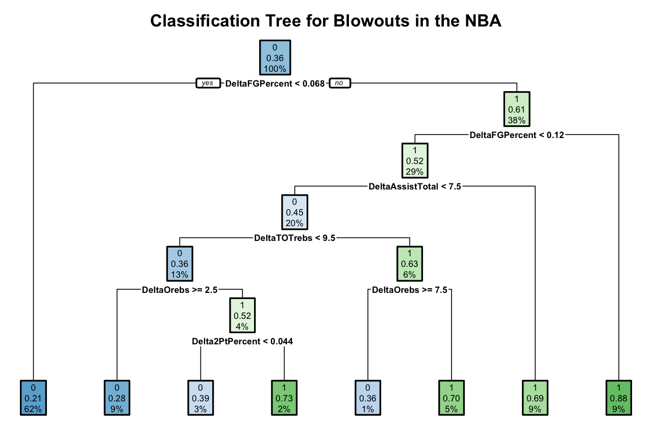
NBA
I made training and test data sets with variables like DeltaTotalAssists, DeltaFieldGoalPercentage, DeltaTurnovers, DeltaOffensiveRebounds, etc. I then created a CART model to predict blowout games by looking at the differentials from these and other basketball game stats.
Each node (or leaf) shows:
the predicted outcome (blowout = 1 or not a blowout = 0)
the predicted probability of a blowout
the percentage of observations in the node
Now let’s see how well our CART model did at making predictions for the test set. We can measure the accuracy of the tree model by creating a confusion matrix.
NBA Tree Model Accuracy = 0.7106798
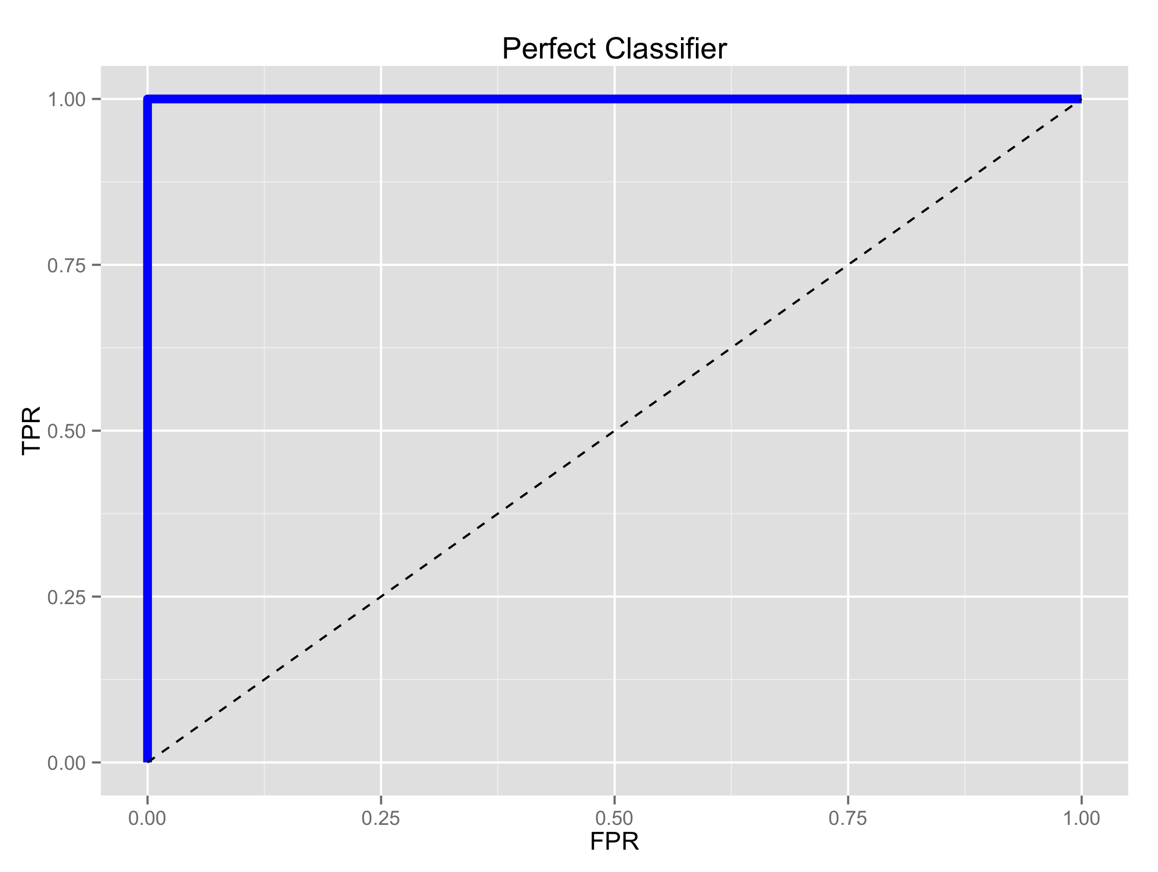
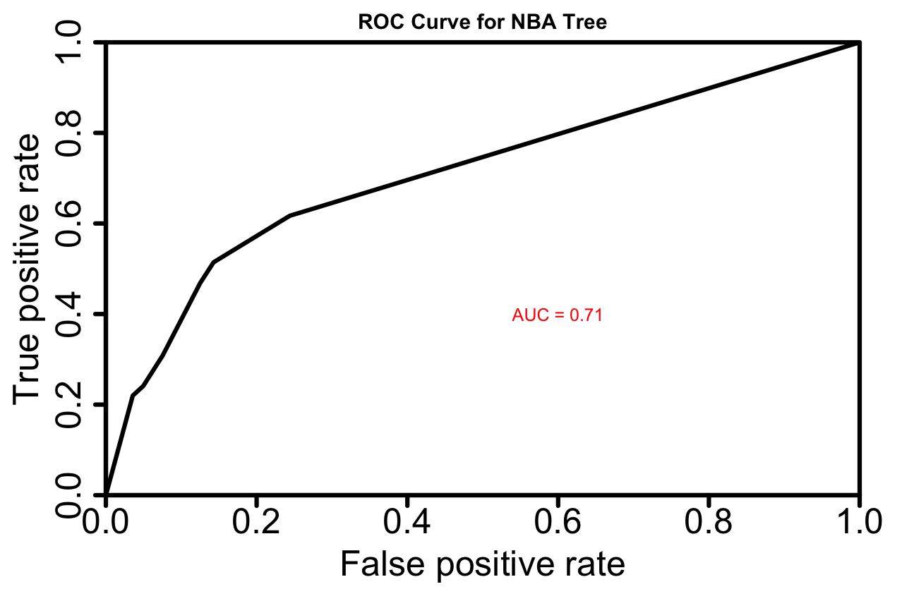
A baseline model that always predicts not a blowout, which is the most common outcome, has an accuracy of 0.6412214. Our NBA CART model is better than baseline. Lastly, let’s generate an ROC curve to evaluate our CART model. The Yhat Blog has a good post explaining ROC curves.
Basically..
This is a perfect model:
This is random guessing:
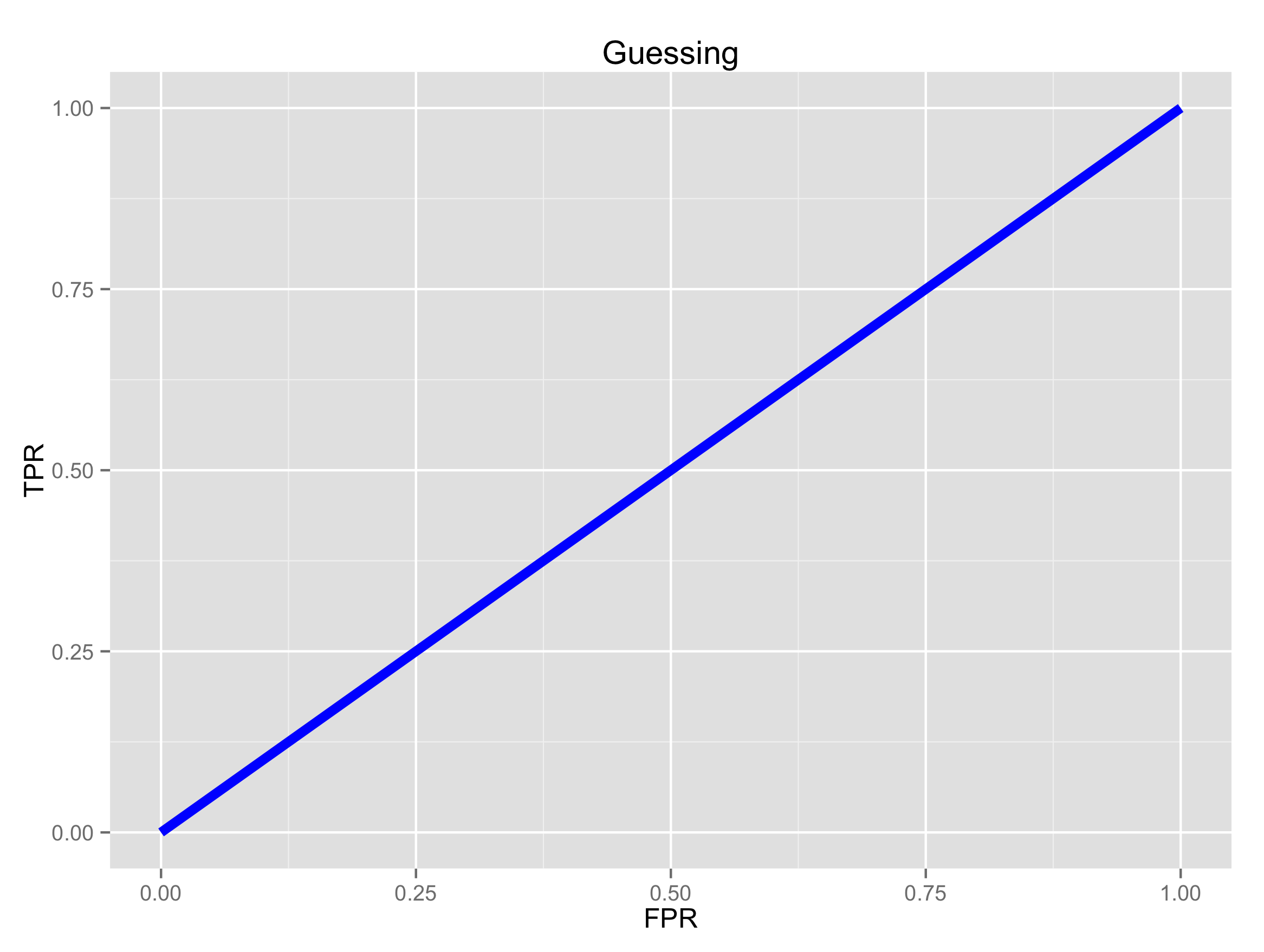
We can calculate an AUC (or area under curve) to quantify how good the model is.
AUC of 1 is good
AUC of .5 is random guessing
NBA ROC Curve
Now that we have a better idea of a CART model and how to quantify its significance, I’ll quickly run through the results for other leagues..
MLB
Each node shows:
the predicted outcome (blowout = 1 or not a blowout = 0)
the predicted probability of a blowout
the percentage of observations in the node
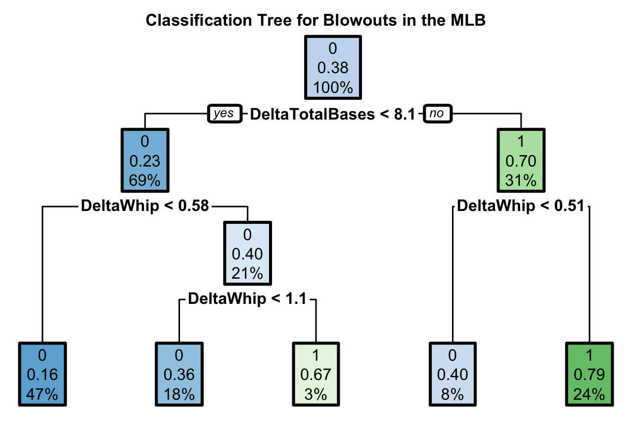
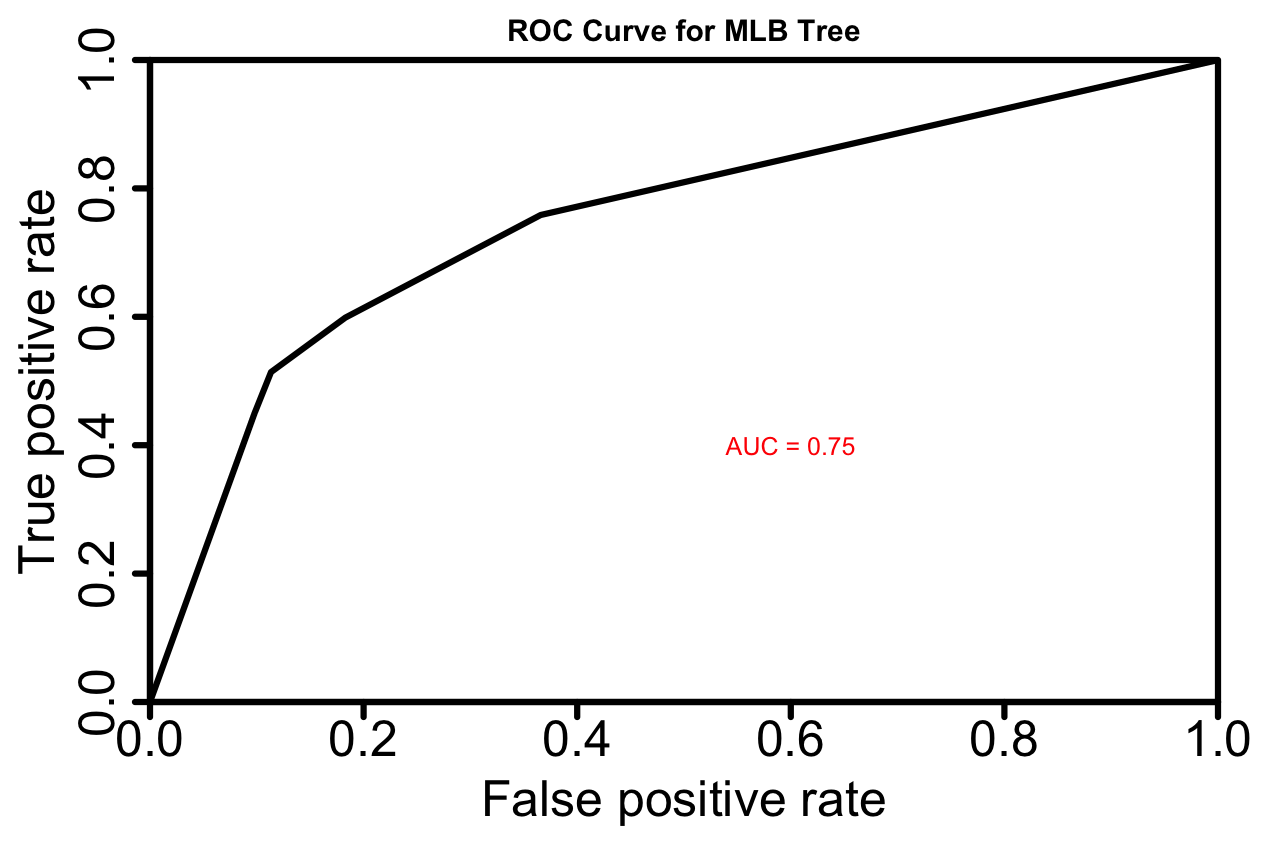
MLB Tree Model Accuracy = 0.7455219
A baseline model that always predicts not a blowout, which is the most common outcome, has an accuracy of 0.6213712. Our MLB CART model is better than baseline.
MLB ROC Curve
NFL
Each node shows:
the predicted outcome (close game = 1 or not a close game = 0)
the predicted probability of a close game
the percentage of observations in the node
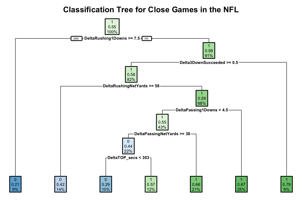
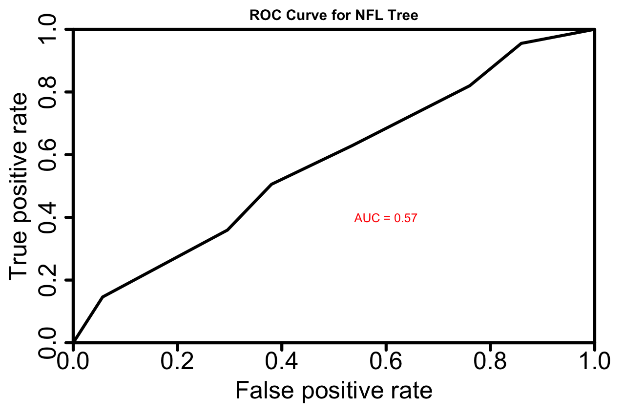
NFL Tree Model Accuracy = 0.5875
A baseline model that always predicts not a close game, which is the most common outcome, has an accuracy of 0.4625. Our NFL CART model is better than baseline but only slightly better than random guessing.
NFL ROC Curve
NHL
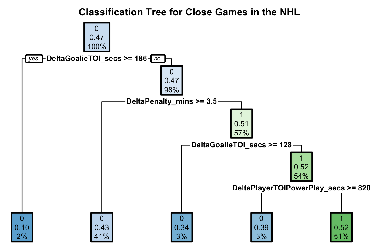
Each node shows:
the predicted outcome (close game = 1 or not a close game = 0)
the predicted probability of a close game
the percentage of observations in the node
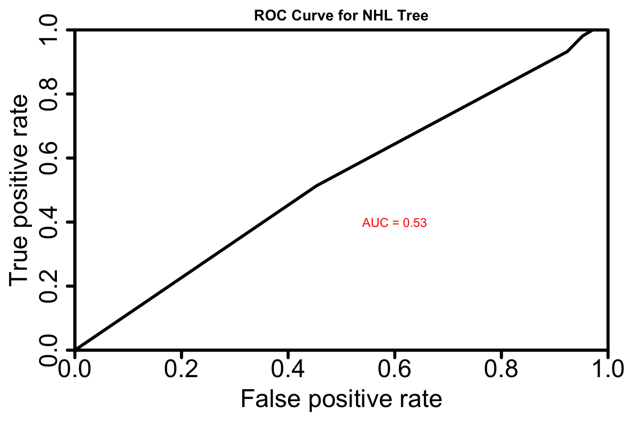
NHL Tree Model Accuracy = 0.531052
A baseline model that always predicts not a close game, which is the most common outcome, has an accuracy of 0.561052. Our NHL CART model is slightly worse than baseline and only slightly better than random guessing.
NHL ROC Curve
| League | CART Model Accuracy |
|---|---|
| MLB | 0.74 |
| NBA | 0.71 |
| NFL | 0.58 |
| NHL | 0.53 |
Random Forest Model
The second method I use is called Random Forest. This method was designed to improve the prediction accuracy of CART and works by building a large number of CART trees. To make a prediction for a new observation, each tree in the forest votes on the outcome and we pick the outcome that receives the majority of the votes.
Using R’s randomForest package, I created a model for each league using the same variables we used for CART. Random Forest model improved the accuracy over the previous CART method for each league. We’ll use these accuracy results in the competitiveIndex calculation.
| League | Random Forest Model Accuracy |
|---|---|
| NBA | 0.77 |
| MLB | 0.75 |
| NFL | 0.60 |
| NHL | 0.60 |
Conclusion
To determine the most and least competitive leagues, I calculated a ‘Competitive Index’ using the results from the analysis.
This index is essentially an average of all values and a measure of competitiveness on a scale of 0 to 1
1 being most competitive
0 being least competitive
| League | competitiveIndex |
|---|---|
| NHL | 0.48 |
| NFL | 0.47 |
| MLB | 0.34 |
| NBA | 0.29 |
And there we have it; the NHL is the most competitive league with competitiveIndex score of 0.48. The NFL is close behind with a score of 0.47. Next, I will create an R Shiny application that will allow us to manipulate the point thresholds for the various categories. For now, thanks for reading and be sure to send me a message with your thoughts.
Update:
May 31st, 2017: This post has been updated with the latest NBA and NHL 2017 playoff outcomes.
June 13th, 2017: This post has been updated with the conclusion of both NBA and NHL 2017 finals.